Hot Routes and Street Profiles

class: center, middle, inverse, title-slide

# Hot Routes and Street Profiles
### Réka Solymosi
### University of Manchester
### 16/05/2022

---

class: center, middle

# My research

- Fear of crime (place-based approach)
- New (?) / alternative (?) forms of data
- Under-reported crimes
- Data visualisation

---
class: middle, center, inverse

# Visualising crime along a network

---
class: middle, center

```r
library(sf)
library(tidyverse)
mcr_roads <- st_read("data/mcr_roads.geojson")
mcr_asb <- st_read("data/mcr_asb.geojson")
ggplot() + 
  geom_sf(data = mcr_roads) + 
  geom_sf(data = mcr_asb, colour = "red") + 
  theme_void()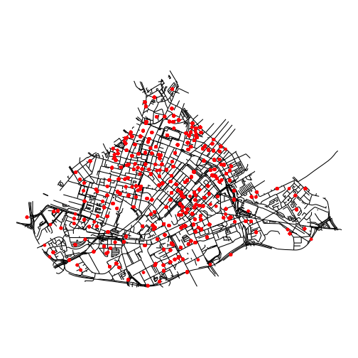
```

![](nscr_talk_files/figure-html/unnamed-chunk-1-1.png)

---
class: middle, center

```r
library(spatstat)
# window
city_centre <- st_read("data/mcr_cc_poly.geojson")
window <- as.owin(city_centre)
# extract coordinates
asb_coords <- matrix(unlist(mcr_asb$geometry), ncol = 2, byrow = T)
# make into pppt 
asb_ppp <- ppp(x = asb_coords[,1], y = asb_coords[,2],
               window = window, check = T)
# jitter because duplicates
jitter_asb <- rjitter(asb_ppp, retry=TRUE, nsim=1, drop=TRUE)
```

---
class: middle, center

```r
plot(density(jitter_asb, sigma = 50))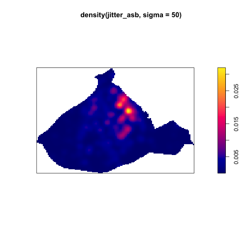
```

![](nscr_talk_files/figure-html/unnamed-chunk-3-1.png)

---
class: middle, center

# Two techniques for visualising along network

- Hot routes
- Street profile

(return to spatstat solution if time)

---
class: middle, center

# Hot routes

- Developed for crime on public transport

> "it is very difficult to pinpoint the location of a crime that occurs on
a moving vehicle" (Newton, 2014)

---
class: middle, center

# Hot routes

- Application for visualisation with GIS

> "devised with the everyday crime analyst in mind" (Tompson, Partridge & Shepherd, 2009)

---
class: middle, center

# 4 stages

- Step 1. Preparing the network layer
- Step 2. Linking crime events to street segments
- Step 3. Calculating a rate
- Step 4. Visualising the results

---
class: middle, center

# Preparing the network layer (1/2)

```r
knitr::kable(mcr_roads[1:3,1:2])
```

|osm_id |name              |geometry                       |
|:------|:-----------------|:------------------------------|
|796680 |Altrincham Street |LINESTRING (384498.2 397606... |
|796758 |Cobourg Street    |LINESTRING (384619.8 397718... |
|797061 |South Pump Street |LINESTRING (384697.8 397780... |

---
class: middle, center

# Preparing the network layer (2/2)

```r
mcr_roads <- rownames_to_column(mcr_roads, "id")
mcr_roads$id <- as.numeric(as.character(mcr_roads$id ))
```

---
class: middle, center

# Linking events to street segments (1/4)

```r
nearest_segments <- st_nearest_feature(mcr_asb, mcr_roads)
```

This new object is simply a list of the ID numbers of matched line segments for each of the ASB incidents. For example here is the ID number of the nearest street segment for the first 5 ASB incidents in our data:

```r
nearest_segments[1:5]
```

```
## [1]  780  254  102 1959 1959
```

---
class: middle, center

# Linking events to street segments (2/4)

We can use this to create a frequency table which counds the number of ASB incidents linked to each street segment (by virtue of being nearest to it)

```r
#make list of nearest into df of frequency
nearest_freq <- as.data.frame(table(nearest_segments))

#make sure id is numeric
nearest_freq$nearest_segments <- as.numeric(as.character(nearest_freq$nearest_segments))

knitr::kable(nearest_freq[1:3,])
```

| nearest_segments| Freq|
|----------------:|----:|
|                2|    8|
|               10|    5|
|               12|    9|

---
class: middle, center

# Linking events to street segments (3/4)

```r
#join to sections object and replace NAs with 0s
mcr_roads <- left_join(mcr_roads, 
                       nearest_freq,
                       by = c("id" = "nearest_segments")) %>% 
  mutate(Freq = replace_na(Freq, 0))

knitr::kable(mcr_roads[1:3,c(1:3,317)])
```

| id|osm_id |name              | Freq|geometry                       |
|--:|:------|:-----------------|----:|:------------------------------|
|  1|796680 |Altrincham Street |    0|LINESTRING (384498.2 397606... |
|  2|796758 |Cobourg Street    |    8|LINESTRING (384619.8 397718... |
|  3|797061 |South Pump Street |    0|LINESTRING (384697.8 397780... |

---
class: middle, center

# Linking events to street segments (4/4)

Quick visualisation to check

```r
p1 <- ggplot() + 
  geom_sf(data = mcr_roads, 
          aes(colour = Freq), lwd = 0.5) + 
  theme_void() +
  scale_colour_gradient2(name = "Number of ASB incidents", 
                         midpoint = 10,
                         low = "#2166ac", 
                         mid = "#d1e5f0", 
                         high = "#b2182b")
```

---
class: middle, center

```r
p1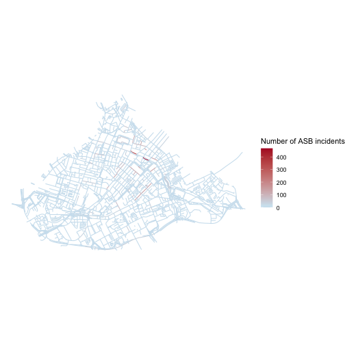
```

![](nscr_talk_files/figure-html/unnamed-chunk-11-1.png)

---
class: middle, center

# Calculating a rate (1/2)

```r
mcr_roads$length <- st_length(mcr_roads)

knitr::kable(mcr_roads[1:3,c(1:3,319)])
```

| id|osm_id |name              |       length|geometry                       |
|--:|:------|:-----------------|------------:|:------------------------------|
|  1|796680 |Altrincham Street | 78.13335 [m]|LINESTRING (384498.2 397606... |
|  2|796758 |Cobourg Street    | 84.60668 [m]|LINESTRING (384619.8 397718... |
|  3|797061 |South Pump Street | 37.47319 [m]|LINESTRING (384697.8 397780... |

---
class: middle, center

# Calculating a rate (2/2)

```r
mcr_roads$asb_per_m <- as.numeric(mcr_roads$Freq / mcr_roads$length)

knitr::kable(mcr_roads[1:3,c(1:3,320)])
```

| id|osm_id |name              | asb_per_m|geometry                       |
|--:|:------|:-----------------|---------:|:------------------------------|
|  1|796680 |Altrincham Street | 0.0000000|LINESTRING (384498.2 397606... |
|  2|796758 |Cobourg Street    | 0.0945552|LINESTRING (384619.8 397718... |
|  3|797061 |South Pump Street | 0.0000000|LINESTRING (384697.8 397780... |

---
class: middle, center

# Visualise the results (1/2)

```r
p1 <- ggplot() + 
  geom_sf(data = mcr_roads, aes(colour = asb_per_m), 
          lwd = 0.5, alpha = 0.8) + 
  theme_void() +
  scale_colour_gradient2(name = "ASB incidents per meter", 
                         midpoint = mean(mcr_roads$asb_per_m),
                         low = "#2166ac", mid = "#d1e5f0", 
                         high = "#b2182b")
```

---
class: middle, center

```r
p1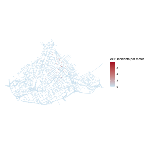
```

![](nscr_talk_files/figure-html/unnamed-chunk-15-1.png)

---
class: middle, center

# Visualise the results (2/2)

```r
p1 <- ggplot() + 
  geom_sf(data = mcr_roads, aes(colour = asb_per_m, size = asb_per_m),
          show.legend = "line", alpha = 0.8) + 
  theme_void() +
  scale_colour_gradient2(name = "ASB incidents per meter", 
                         midpoint = mean(mcr_roads$asb_per_m),
                         low = "#2166ac", mid = "#d1e5f0", high = "#b2182b") +
  scale_size_continuous(name = "ASB incidents per meter (width)") 
```

---
class: middle, center

```r
p1
```

![](nscr_talk_files/figure-html/unnamed-chunk-17-1.png)

---
class:middle, center

# The spatstat way

(this is a density plot rather than hot route though... )

```r
library(maptools)
# make mcr_roads into sp object
mcr_roads_sp <- as(mcr_roads, 'Spatial')
# turn into line network (linnet)
mcr_roads_linnet <- as.linnet.SpatialLines(mcr_roads_sp)
# now use this and previously created linnet to make lpp object
asb_lpp <- lpp(jitter_asb, mcr_roads_linnet)
```

---
class:middle, center

# Calculate density and visualise

```r
# calculate density
d150 <- density.lpp(asb_lpp, 150, finespacing=FALSE)

# plot
plot(d150)
```

![](nscr_talk_files/figure-html/unnamed-chunk-19-1.png)

---
class: middle, center

# Or visualise with line width

```r
# plot
plot(d150, style="width")
```

![](nscr_talk_files/figure-html/unnamed-chunk-20-1.png)

---
class: center, middle

# Street profile analysis

[Spicer et al., 2016](https://www.sciencedirect.com/science/article/pii/S0143622816300170)
- method for visualising temporal and spatial crime patterns along major roadways
- geographical location of the street may not be important
- treat the street in question as the x-axis of a graph, with a start point (A) and end point (B)

---
class: center, middle

# Street profile analysis

- Step 1: Prepare the network layer
- Step 2. Link crime events to points of interest
- Step 3: Calculate a rate
- Step 4: Visualise the results

---
class: middle, center

# Preparing the network layer (1/2)

```r
# we select a busy street
deansgate <- mcr_roads %>% filter(name == "Deansgate") %>% 
  select(id, name, length, geometry, asb_per_m)

# and select also the cross streets into separate object
dg_intersects <- st_intersects(deansgate, mcr_roads)
# subsetting
dg_intersects <- mcr_roads[unlist(dg_intersects),]
```

---
class: middle, center

# Plot for a visual check (2/2)

```r
p1 <- ggplot() + 
  geom_sf(data = dg_intersects, lwd = 0.5) + 
  geom_sf(data = deansgate, aes(colour = as.character(id)), lwd = 1.5, alpha = 0.8) + 
  geom_sf(data = deansgate %>% filter(id == 167), colour = "red", lwd = 3) + 
  theme_void() + theme(legend.position = "none")
```

---
class: middle, center

```r
p1
```

![](nscr_talk_files/figure-html/unnamed-chunk-23-1.png)

---
class: middle, center

# Linking events to street segments (1/3)

```r
# select only offences in May and then link as we did before with
#   st_nearest_feature()
mcr_asb_may <- mcr_asb %>% filter(month == "2016-05")
nearest_segments_may <- st_nearest_feature(mcr_asb_may, mcr_roads)
nearest_freq_may <- as.data.frame(table(nearest_segments_may))
nearest_freq_may <- nearest_freq_may %>% 
  mutate(nearest_segments_may = as.numeric(as.character(nearest_freq_may$nearest_segments_may))) %>% 
  rename(may_asb = Freq)
deansgate <- left_join(deansgate, 
                       nearest_freq_may,
                       by = c("id" = "nearest_segments_may")) %>% 
  mutate(may_asb = replace_na(may_asb, 0)) 
```

---
class: middle, center

# Linking events to street segments (2/3)

```r
# Do it again for June
mcr_asb_jun <- mcr_asb %>% filter(month == "2016-06")
nearest_segments_june <- st_nearest_feature(mcr_asb_jun, mcr_roads)
nearest_freq_june <- as.data.frame(table(nearest_segments_june))
nearest_freq_june <- nearest_freq_june %>% 
  mutate(nearest_segments_june = as.numeric(as.character(nearest_freq_june$nearest_segments_june))) %>% 
  rename(june_asb = Freq)
deansgate <- left_join(deansgate, 
                       nearest_freq_june,
                       by = c("id" = "nearest_segments_june")) %>% 
  mutate(june_asb = replace_na(june_asb, 0)) 
```

---
class: middle, center

# Linking events to street segments (3/3)

Quick visualisation to check

```r
p1 <- ggplot() + 
  geom_sf(data = deansgate, aes(colour = may_asb), lwd = 0.5) + 
  theme_void() +
  scale_colour_gradient2(name = "May ASB", 
                         midpoint = 1,
                         low = "#2166ac", mid = "#d1e5f0", high = "#b2182b")

p2 <- ggplot() + 
  geom_sf(data = deansgate, aes(colour = june_asb), lwd = 0.5) + 
  theme_void() +
  scale_colour_gradient2(name = "June ASB", 
                         midpoint = 1,
                         low = "#2166ac", mid = "#d1e5f0", high = "#b2182b")
```

---
class: middle, center

```r
gridExtra::grid.arrange(p1,p2, nrow = 1)
```

![](nscr_talk_files/figure-html/unnamed-chunk-27-1.png)

---
class: middle, center

# Calculating a rate (1/1)

(we have length from calculating for hot routes)

```r
deansgate$may_rate <- as.numeric(deansgate$may_asb / deansgate$length)
deansgate$june_rate <- as.numeric(deansgate$june_asb / deansgate$length)
```

---
class: middle, center

# Visualise (1/7)

Need order - so find "point A". Here I know it's id = 167. And calculate distance for each other segment

```r
datalist <- list()
i <- 1
for(segment_id in deansgate$id){

datalist[[i]] <- data.frame(id = segment_id, 
                              dist_from_a = st_distance(
                                deansgate %>% filter(id == 167),
                                deansgate %>%  filter(id == segment_id)))
i <- i + 1  
}

dist_matrix <- do.call(rbind, datalist)

deansgate <- left_join(deansgate, dist_matrix)
```

```
## Joining, by = "id"
```

---
class: middle, center

# Visualise (2/7)

```r
p1 <- ggplot(deansgate, aes(x = reorder(as.character(id), 
                                  dist_from_a), 
                      y = may_asb, 
                      group = name)) + 
  geom_point() + 
  geom_line() + 
  xlab("Deansgate") + 
  ylab("ASB incidents") + 
  theme_bw() + 
  theme(axis.text.x = element_text(angle = 60, hjust = 1))
```

---
class: middle, center

```r
p1
```

![](nscr_talk_files/figure-html/unnamed-chunk-31-1.png)

---
class: middle, center

# Visualise (3/7)

Get names of cross streets

```r
# filter deansgate itself and NA names
x_streets <- dg_intersects %>% 
  filter(name != "Deansgate" &
           !is.na(name)) %>% 
  mutate(xst_id = 1:nrow(.))
```

---
class: middle, center

# Visualise (4/7)

Find nearest intersecting street for each segment

```r
datalist <- list()
i <- 1
for(segment_id in deansgate$id){

datalist[[i]] <- data.frame(id = segment_id,
                    x_street = st_nearest_feature(
                      deansgate %>%
                        filter(id == segment_id), x_streets))
i <- i + 1  
}

nearest_matrix <- do.call(rbind, datalist)
```

---
class: middle, center

# Visualise (5/7)

Get names of cross streets

```r
nearest_matrix <- left_join(nearest_matrix,
                            x_streets %>% 
                              select(xst_id, name) %>%
                              st_drop_geometry(),
                            by = c('x_street' = 'xst_id'))

deansgate <- left_join(deansgate, nearest_matrix, 
                       by = c("id" = "id")) %>% 
  mutate(name.y = make.unique(name.y))
```

---
class: middle, center

# Visualise (6/7)

```r
p1 <- ggplot(deansgate, aes(x = reorder(name.y, 
                                  dist_from_a), 
                      y = may_asb, 
                      group = name.x)) + 
  geom_point() + 
  geom_line() + 
  xlab("Deansgate") + 
  ylab("ASB incidents") + 
  theme_bw() + 
  theme(axis.text.x = element_text(angle = 60, hjust = 1))
```

---
class: center, middle

```r
p1
```

![](nscr_talk_files/figure-html/unnamed-chunk-36-1.png)

---
class: middle, center

# Visualise (7/7)

```r
p1 <- ggplot() + 
  geom_point(data = deansgate, aes(x = reorder(name.y, 
                                  dist_from_a), 
                      y = may_asb, group = name.x), col = "#2166ac") + 
  geom_line(data = deansgate, aes(x = reorder(name.y, 
                                  dist_from_a), 
                      y = may_asb, group = name.x), col = "#2166ac") + 
    geom_point(data = deansgate, aes(x = reorder(name.y, 
                                  dist_from_a), 
                      y = june_asb, group = name.x), col = "#b2182b") + 
  geom_line(data = deansgate, aes(x = reorder(name.y, 
                                  dist_from_a), 
                      y = june_asb, group = name.x), col = "#b2182b") + 
  scale_colour_manual(values = c("#2166ac", "#b2182b"), 
                      labels = c("May", "June")) +
  xlab("Deansgate") +  ylab("ASB incidents") + theme_bw() + 
  theme(axis.text.x = element_text(angle = 60, hjust = 1)) +
  guides(colour = guide_legend(title = "Month")) 
```

---
class: middle, center

```r
p1
```

![](nscr_talk_files/figure-html/unnamed-chunk-38-1.png)

---
class: center, middle

# Relevant Papers

- [Street profile analysis: A new method for mapping crime on major roadways](https://www.sciencedirect.com/science/article/abs/pii/S0143622816300170)
- [Hot Routes JDI brief ](https://www.ucl.ac.uk/jill-dando-institute/sites/jill_dando_institute/files/hot_routes_1-5_all.pdf)
- [Hot Routes: Developing a New Technique for the Spatial Analysis of Crime  ](https://discovery.ucl.ac.uk/id/eprint/20057/)