Overview

• Brief introduction to the importance of data analysis in criminology

• Overview of R as an open-source programming language and software environment

• Advantages of R

• Examples of utility

• How to get started

• Practice example

• Q & A

The importance of data analysis in criminology

• Academic Research and Theoretical Development

• Understanding Crime Patterns

• Informed Decision-Making

• Evaluation of Criminal Justice Policies

• Interdisciplinary Applications

• and so on...

So why R?

Reason 1: Open source

Free (accessible)

• For students, teachers, professionals
• No licence required
• Download R: https://www.r-project.org/
• Download R Studio (IDE): https://posit.co/downloads/

Many contributors (range of packages)

• Any type of analysis you want to do - it is possible
• Anyone can contribute
• If it doesn't exist, someone will write it

Community support

https://stackoverflow.com/questions/57675328/neighbour-list-with-poly2nb-works-on-2004-census-shapefile-but-not-on-2011

Community support

Community support

Community support

Community support

Reason 2: Versatile

Data

library(fivethirtyeight)
head(hate_crimes)

##        state state_abbrev median_house_inc share_unemp_seas share_pop_metro
## 1    Alabama           AL            42278            0.060            0.64
## 2     Alaska           AK            67629            0.064            0.63
## 3    Arizona           AZ            49254            0.063            0.90
## 4   Arkansas           AR            44922            0.052            0.69
## 5 California           CA            60487            0.059            0.97
## 6   Colorado           CO            60940            0.040            0.80
##   share_pop_hs share_non_citizen share_white_poverty gini_index share_non_white
## 1        0.821              0.02                0.12      0.472            0.35
## 2        0.914              0.04                0.06      0.422            0.42
## 3        0.842              0.10                0.09      0.455            0.49
## 4        0.824              0.04                0.12      0.458            0.26
## 5        0.806              0.13                0.09      0.471            0.61
## 6        0.893              0.06                0.07      0.457            0.31
##   share_vote_trump hate_crimes_per_100k_splc avg_hatecrimes_per_100k_fbi
## 1             0.63                0.12583893                   1.8064105
## 2             0.53                0.14374012                   1.6567001
## 3             0.50                0.22531995                   3.4139280
## 4             0.60                0.06906077                   0.8692089
## 5             0.33                0.25580536                   2.3979859
## 6             0.44                0.39052330                   2.8046888

Analysis

library(skimr)
skim(hate_crimes)

Summary stats

summary_hate_crimes <- summary(hate_crimes$hate_crimes_per_100k_splc)
summary_hate_crimes

##    Min. 1st Qu.  Median    Mean 3rd Qu.    Max.    NA's 
## 0.06745 0.14271 0.22620 0.30409 0.35694 1.52230       4

T-test

# Create a new variable to categorise states
hate_crimes$income_category <- ifelse(hate_crimes$median_house_inc > median(hate_crimes$median_house_inc), "High", "Low")
# Perform a t-test
t_test_result <- t.test(hate_crimes$hate_crimes_per_100k_splc ~ hate_crimes$income_category)
t_test_result

## 
##     Welch Two Sample t-test
## 
## data:  hate_crimes$hate_crimes_per_100k_splc by hate_crimes$income_category
## t = 2.1658, df = 27.187, p-value = 0.03926
## alternative hypothesis: true difference in means between group High and group Low is not equal to 0
## 95 percent confidence interval:
##  0.008498125 0.312551012
## sample estimates:
## mean in group High  mean in group Low 
##          0.3894784          0.2289538

Missing values

missing_values <- sum(is.na(hate_crimes$hate_crimes_per_100k_splc))
missing_values

## [1] 4

Calculate correlation

correlation <- cor.test(hate_crimes$median_house_inc, 
                   hate_crimes$hate_crimes_per_100k_splc, 
                   use = "complete.obs", 
                   method = "pearson")
correlation

## 
##     Pearson's product-moment correlation
## 
## data:  hate_crimes$median_house_inc and hate_crimes$hate_crimes_per_100k_splc
## t = 2.5122, df = 45, p-value = 0.01565
## alternative hypothesis: true correlation is not equal to 0
## 95 percent confidence interval:
##  0.07066435 0.57951602
## sample estimates:
##       cor 
## 0.3507143

Calculate regression

# Fit a linear regression model
model <- lm(hate_crimes_per_100k_splc ~ median_house_inc + 
              share_vote_trump + 
              share_non_citizen, 
            data = hate_crimes)
summary(model)

## 
## Call:
## lm(formula = hate_crimes_per_100k_splc ~ median_house_inc + share_vote_trump + 
##     share_non_citizen, data = hate_crimes)
## 
## Residuals:
##      Min       1Q   Median       3Q      Max 
## -0.35450 -0.11333 -0.04116  0.08900  0.50329 
## 
## Coefficients:
##                     Estimate Std. Error t value Pr(>|t|)    
## (Intercept)        1.626e+00  3.996e-01   4.068  0.00021 ***
## median_house_inc  -4.351e-06  4.122e-06  -1.056  0.29729    
## share_vote_trump  -2.006e+00  3.880e-01  -5.169  6.5e-06 ***
## share_non_citizen -2.083e+00  1.149e+00  -1.814  0.07707 .  
## ---
## Signif. codes:  0 '***' 0.001 '**' 0.01 '*' 0.05 '.' 0.1 ' ' 1
## 
## Residual standard error: 0.1881 on 41 degrees of freedom
##   (6 observations deleted due to missingness)
## Multiple R-squared:  0.4791,    Adjusted R-squared:  0.441 
## F-statistic: 12.57 on 3 and 41 DF,  p-value: 5.751e-06

Present results nicely

library(broom)
# Tidy the model results
tidy_model <- tidy(model)
# Print the tidy model as an HTML table
tidy_model %>%
  knitr::kable("html", caption = "Regression Results") %>%
  kableExtra::kable_styling(full_width = FALSE)

library(sjPlot)
# Create a forest plot for the regression model
plot_model(model, type = "est", show.values = TRUE, show.ci = TRUE) +
  labs(title = "Forest Plot of Regression Coefficients", x = "Estimate", y = "Predictors")

Many types of analysis

Network

# Load the libraries
library(igraph)
library(igraphdata)
# Load a sample network dataset
data("USairports")
# Plot the network graph
plot(USairports, 
     vertex.size=5, 
     vertex.label=NA, 
     edge.arrow.size=0.3, 
     main="US Airports Network")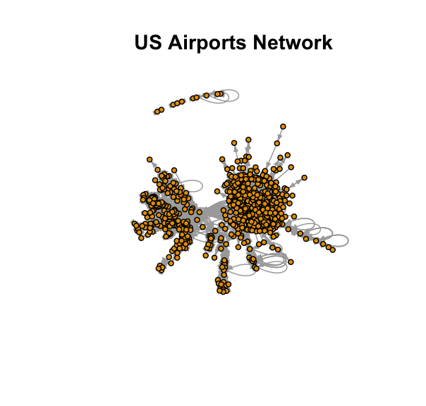

Spatial

# Load the library
library(tmap)
# Load the inbuilt dataset
data("World")
# Create a quick map
tm_shape(World) + 
  tm_polygons("pop_est", 
              title = "Population") +
  tm_layout(main.title = "World Population Map", 
            frame = FALSE)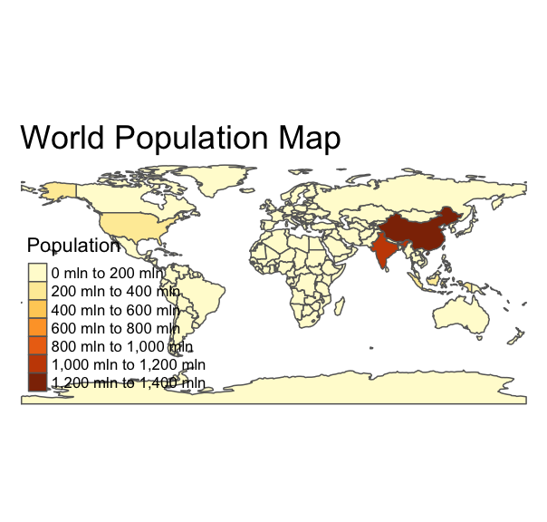

Text

# Load the libraries
library(wordcloud)
library(tm)
# Load a sample text dataset
data("crude")
# Create a term-document matrix
tdm <- TermDocumentMatrix(crude)
# Convert the matrix to a format for word cloud
m <- as.matrix(tdm)
word_freq <- sort(rowSums(m), 
                  decreasing=TRUE)
# Generate the word cloud
wordcloud(names(word_freq), 
          word_freq, max.words=100)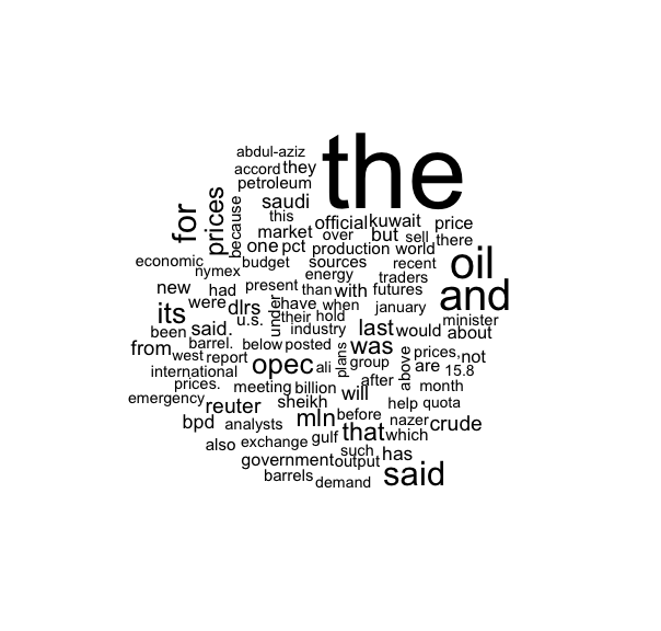

Machine learning

# Load the libraries
library(rpart)
library(ggparty)
# Load the dataset
data(iris)
# Create a decision tree model using rpart directly
model <- rpart(Species ~ ., data = iris)

More ML

library(caret)
# Load the iris dataset
data(iris)
# Split the data into training and testing sets (70% training, 30% testing)
set.seed(123)
trainIndex <- createDataPartition(iris$Species, p = 0.7, list = FALSE)
trainData <- iris[trainIndex, ]
testData <- iris[-trainIndex, ]
# Train a KNN model
model <- train(Species ~ ., data = trainData, method = "knn", tuneLength = 5)
# Predict on the test data
predictions <- predict(model, testData)
# Evaluate the model with a confusion matrix
confusionMatrix(predictions, testData$Species)

## Confusion Matrix and Statistics
## 
##             Reference
## Prediction   setosa versicolor virginica
##   setosa         15          0         0
##   versicolor      0         14         1
##   virginica       0          1        14
## 
## Overall Statistics
##                                           
##                Accuracy : 0.9556          
##                  95% CI : (0.8485, 0.9946)
##     No Information Rate : 0.3333          
##     P-Value [Acc > NIR] : < 2.2e-16       
##                                           
##                   Kappa : 0.9333          
##                                           
##  Mcnemar's Test P-Value : NA              
## 
## Statistics by Class:
## 
##                      Class: setosa Class: versicolor Class: virginica
## Sensitivity                 1.0000            0.9333           0.9333
## Specificity                 1.0000            0.9667           0.9667
## Pos Pred Value              1.0000            0.9333           0.9333
## Neg Pred Value              1.0000            0.9667           0.9667
## Prevalence                  0.3333            0.3333           0.3333
## Detection Rate              0.3333            0.3111           0.3111
## Detection Prevalence        0.3333            0.3333           0.3333
## Balanced Accuracy           1.0000            0.9500           0.9500

Sentiment analysis

# Load the libraries
library(tidytext)
library(janeaustenr)
library(dplyr)
library(ggplot2)
# Load the dataset and convert it to a tidy format
data("austen_books")
tidy_books <- austen_books() %>%
  unnest_tokens(word, text)
# Perform sentiment analysis using the Bing lexicon
sentiments <- tidy_books %>%
  inner_join(get_sentiments("bing")) %>%
  group_by(book, sentiment) %>% 
  count()

Plotting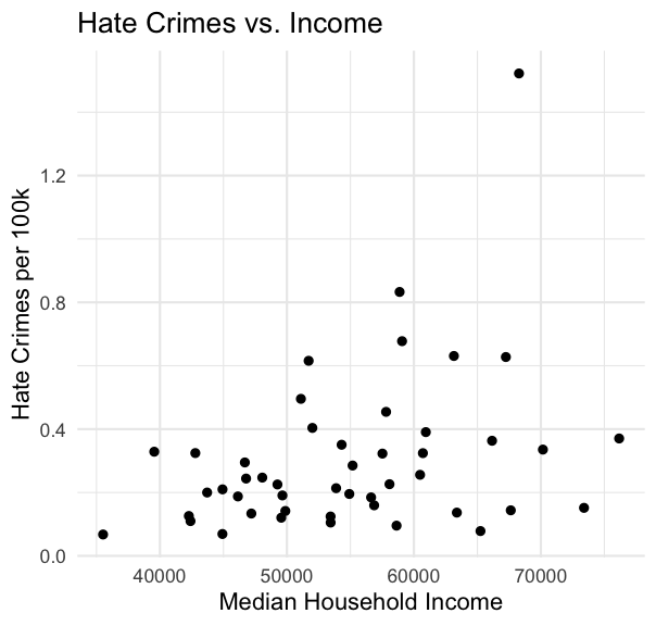

Reason 3: Reproducibility

For open science

• Enhances Transparency: Open science promotes transparency in research methods and data, allowing for better scrutiny and validation of findings.

• Fosters Collaboration: Sharing data and methodologies encourages collaboration among criminologists, leading to more comprehensive studies.

• Accelerates Innovation: Open access to research can accelerate the development of new theories and approaches in criminology.

• Key Resources

  • CrimRxiv: An open-access preprint repository for the criminology community: https://www.crimrxiv.com/
  • Open Science Working Group at the ESC:https://esc-enoc.github.io/

For yourself (e.g., changes for reviewer or repeat analysis/batch processing)

# Scatter plot with regression line
ggplot(hate_crimes, 
       aes(x = median_house_inc, 
           y = hate_crimes_per_100k_splc, 
           color = share_pop_metro)) +
  geom_point() +
  geom_smooth(method = "lm", 
              se = FALSE, 
              color = "black") +
  labs(title = "Hate Crimes vs.Income",
       x = "Median Household Income",
       y = "Hate Crimes per 100k",
       color = "Population Share (Metro)") +
  theme_minimal() +
  scale_color_gradient(low = "grey90", 
                       high = "black")

Less point and click = more transparency, less space for errors

• In 2010, economists Carmen Reinhart and Kenneth Rogoff published a paper titled "Growth in a Time of Debt."
• The paper claimed that countries with debt levels above 90% of GDP experienced slower economic growth.
• A spreadsheet error in their data analysis led to faulty conclusions.
• The findings influenced austerity measures globally, including in the EU and the US.
• Policymakers used the conclusions to justify harsh budget cuts and economic policies.
• See: https://www.bbc.com/news/magazine-22223190

Beyond analysis...

• Slides/ reporting (demo next)
• Websites
• Books

Is it R?

• these slides?
• rekadata.net

• This ESC presentation

• This book

Getting Started with R

• R for Data Science: A free online book that’s an excellent resource for learning R and data science workflows.
• Hands-On Programming with R: Friendly intro to R language for non-programmers
• DataCamp: Introduction to R: Free course offering an interactive way to learn R basics.

Visualisation

• Data Visualization: A practical introduction: Beautiful book on data visualisation
• ggplot2: Elegant Graphics for Data Analysis: A resource for those interested to understand the logic of the Grammar of Graphics that ggplot2 uses.

R Resources for Criminology/ Social Science

• Quantitative Social Science: An Introduction: My favourite social science stats textbook - also uses R
• Discovering Statistics Using R: Very comprehensive, from field of psychology
• A Beginner’s Guide to Statistics for Criminology and Criminal Justice Using R: Written as a companion to classic stats book by Weisburd and Britt
• R for Criminologists: Our course material for PGT
• R for Criminologists: Our course material for UG

Additional Learning

• Stack Overflow: Get help from the R community by browsing or asking questions.
• R Bloggers: Collection of blogs about using R in a variety of disciplines, including criminology.
• Twitter (or maybe Blue Sky now? I don't know!!!)

Demo

Exercise

Code to copy:

# Install necessary packages if they are not already installed
if(!require(ggplot2)) 
  install.packages("ggplot2", dependencies = TRUE)
if(!require(fivethirtyeight)) 
  install.packages("fivethirtyeight", dependencies = TRUE)
# Load the packages
library(ggplot2)
library(fivethirtyeight)
# Create a basic scatter plot of median_house_inc vs. hate_crimes_per_100k_splc
ggplot(hate_crimes, 
       aes(x = median_house_inc, 
           y = hate_crimes_per_100k_splc)) +
  geom_point(color = "blue", 
             size = 3, 
             alpha = 0.6) +  # Scatter plot with blue points
  labs(title = "Hate Crimes per 100k vs. Median Household Income",
       x = "Median Household Income",
       y = "Hate Crimes per 100k") +
  theme_minimal()  # Apply minimal theme for a clean look

Exercise 1: Change the Aesthetics

• Task: Modify the color, size, or transparency of the points in the scatter plot.
• Hint: Use color, size, and alpha arguments in geom_point().

Answer:

# Modify color and size of points
ggplot(hate_crimes, aes(x = median_house_inc, 
                        y = hate_crimes_per_100k_splc)) +
  geom_point(color = "red", size = 5, alpha = 0.8) +  
  labs(title = "Modified Scatter Plot", 
       x = "Median Household Income", 
       y = "Hate Crimes per 100k") +
  theme_minimal()

Exercise 2: Add a Regression Line

• Task: Add a linear regression line to the scatter plot to show the trend.
• Hint: Use geom_smooth() with method = "lm" to add a linear model.

Answer:

# Scatter plot with a regression line
ggplot(hate_crimes, 
       aes(x = median_house_inc, 
           y = hate_crimes_per_100k_splc)) +
  geom_point(color = "blue", size = 3, alpha = 0.6) +
  geom_smooth(method = "lm", color = "black", se = FALSE) +  
  labs(title = "Scatter Plot with Regression Line", 
       x = "Median Household Income", 
       y = "Hate Crimes per 100k") +
  theme_minimal()

Exercise 3: Group Points by a Third Variable

• Task: Color the points by a third variable such as share_pop_metro to explore how urban/rural distribution affects the relationship.
• Hint: Use color = share_pop_metro inside the aes() function.

Answer:

# Scatter plot with points colored by share_pop_metro
ggplot(hate_crimes, 
       aes(x = median_house_inc, 
           y = hate_crimes_per_100k_splc, 
           color = share_pop_metro)) +
  geom_point(size = 3, alpha = 0.6) +
  labs(title = "Scatter Plot by Population",
       x = "Median Household Income", 
       y = "Hate Crimes per 100k", 
       color = "Share Pop Metro") +
  theme_minimal() +
  scale_color_gradient(low = "blue", high = "red")

Exercise 4: Customize the Plot Theme

• Task: Explore different ggplot2 themes such as theme_classic(), theme_bw(), or even modify axis titles, labels, and legend positions.
• Hint: Use theme() to customize the plot or apply pre-built themes like theme_classic().

Answer:

# Custom theme applied to scatter plot
ggplot(hate_crimes, aes(x = median_house_inc, y = hate_crimes_per_100k_splc, color = share_pop_metro)) +
  geom_point(size = 3, alpha = 0.6) +
  labs(title = "Scatter Plot with Custom Theme",
       x = "Median Household Income", y = "Hate Crimes per 100k", color = "Share Pop Metro") +
  theme_classic() +
  theme(plot.title = element_text(hjust = 0.5, size = 14),
        axis.title = element_text(size = 12),
        legend.position = "bottom")

Thank you

Contact: reka.solymosi@manchester.ac.uk