About me

Crime Mapping

Forthcoming textbook based on our UoM Crime Mapping module:

So we see maps everywhere

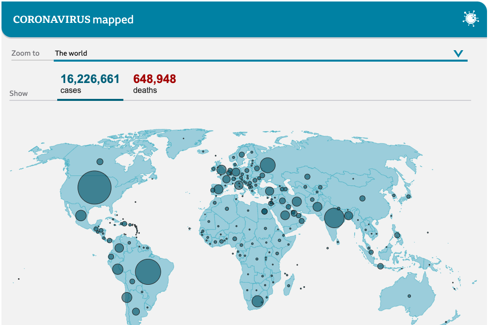
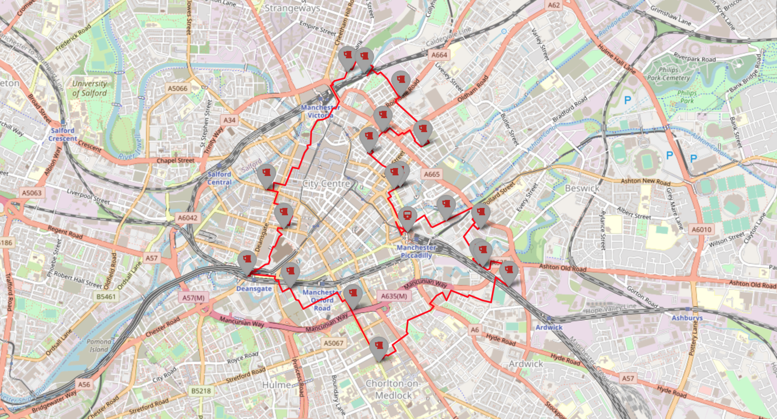
Some are very useful!

Optimal Manchester brewery crawl (see https://www.ncalvert.uk/posts/drunkensalesman/)

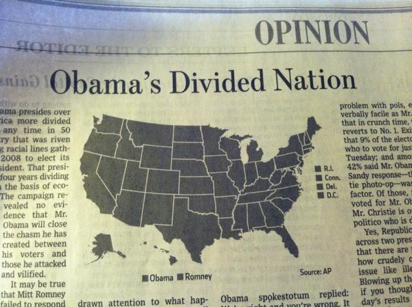
But many are bad

Obligatory XKCD

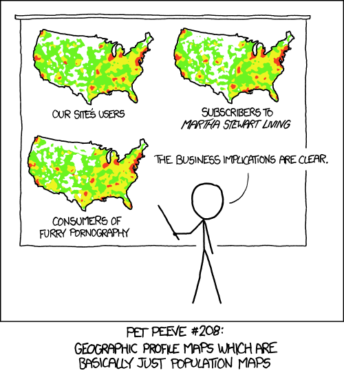
Sometimes bad maps are funny

Some people collect bad maps

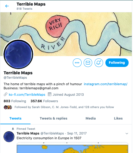
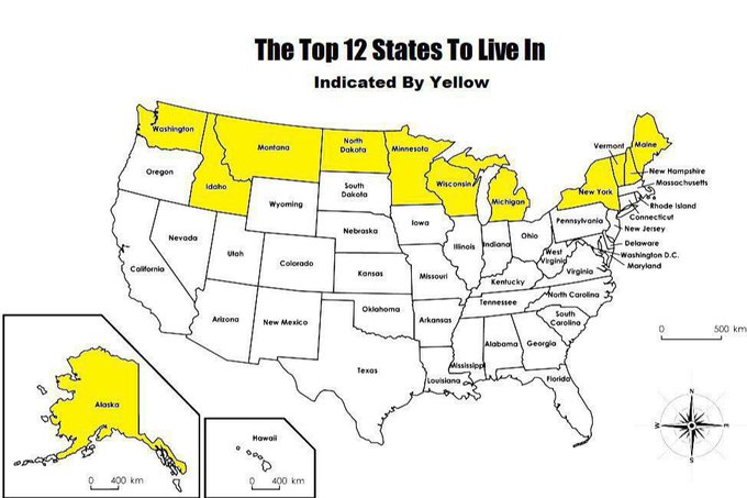
Terrible(/y funny) maps

Two key fields

Example 1: Pie charts

Image credit: Robert Kosara

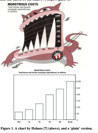
Example 2: Tufte charts

Image credit: Bateman, S., Mandryk, R. L., Gutwin, C., Genest, A., McDine, D., & Brooks, C. (2010, April). Useful junk? The effects of visual embellishment on comprehension and memorability of charts. In Proceedings of the SIGCHI conference on human factors in computing systems (pp. 2573-2582).

Examples in cartography

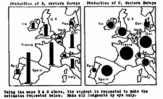
Image credit: Flannery, JJ (1971) The relative effectiveness of some common graduated point symbols in the presentation of quantitative data

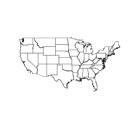
Eg: USA States

Eg: UK Local Authorities

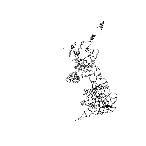
Message often obscured

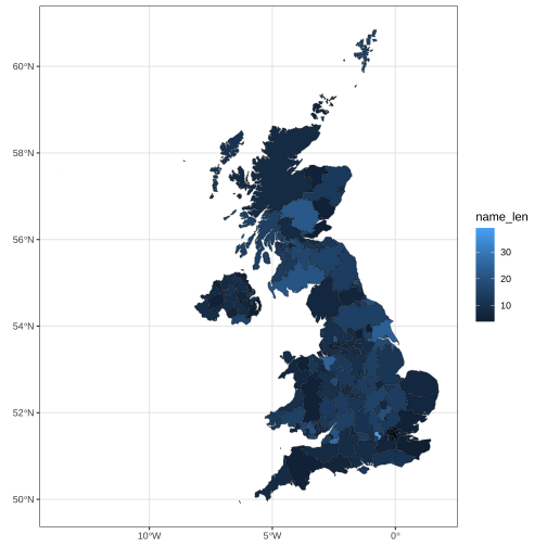
A fix: distort polygons

Our focus: EU referendum results

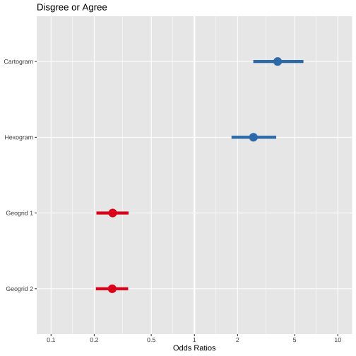
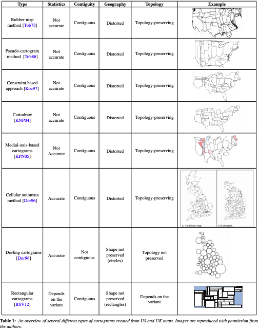
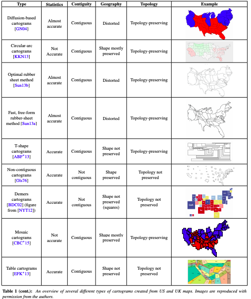
4 types of distortions

(a) Balanced cartogram

• From Harris, R (2017) Hexograms: Better maps of area based data.

• Scale by min value to balance invisibility and distortion

• Eg if SIU is 0.02 inches on a 5inch map:

siu <- 0.02 # the smallest interpretable unit
height <- 5
bb <- sp::bbox(map)
width <- (bb[1,2] - bb[1,1]) / (bb[2,2] - bb[2,1]) * height
bbA <- (bb[1,2] - bb[1,1]) * (bb[2,2] - bb[2, 1])
mapA <- rgeos::gArea(map)
minA <- (siu * bbA) / (height * width)
map$scaleby <- rgeos::gArea(map, byid = TRUE)
map$scaleby[map$scaleby < minA] <- minA
# Use this to scale cartogram
balcarto <- cartogram::cartogram(map, "scaleby", maxSizeError = 1.1, prepare = "none")

(b) Hexogram

• same idea as balanced carto, with minimum value being what allows each area to be represented as its own hexagon

• hexagons are produced using the hexagonal binning function in R’s fMultivar package, based on the centroids of each polygon

• our example:

# Get the function needed
script <- RCurl::getURL("https://raw.githubusercontent.com/profrichharris/Rhexogram/master/functions.R")
eval(parse(text = script))
# Number of bins guided by the -binN- function for a visual plot.
# 29 is also used by Harris in example.
harris.29  <- hexogram(LAE.sp, 29)
# Extract the hexograms
harris.29.hex.sp <- harris.29[[2]]   # 2 is hexo

(c) geogrid squre grid

• From Joseph Bailey

• Calculates a grid that strives to preserve the original geography.

• 2 steps to using this

  • 1 - Generate grid by varying the seed

  • 2 - Efficiently calculate the assignments from the original geography to the new geography

• Our example:

# step 1 generate grid
LAE.reg <- calculate_grid(shape = LAE.sp, grid_type = "regular", seed = 1) #1 was our fave seed
# step 2 calculate assignments
LAE.reg <- assign_polygons(LAE.sp, LAE.reg)

(d) geogrid hexagonal grid

• Same idea as with grids but for hexagons:

# step 1 generate grid
LAE.hex <- calculate_grid(shape = LAE.sp, grid_type = "hexagonal", seed = 1)
# step 2 calculate assignments
LAE.hex <- assign_polygons(LAE.sp, LAE.hex)

- 5-point Likert scale (strongly agree, slightly agree, neither agree nor disagree, slightly disagree, strongly disagree).

• Higher agreement = better representation of statement in map

• Convenience sample (internet) of 768 respondents

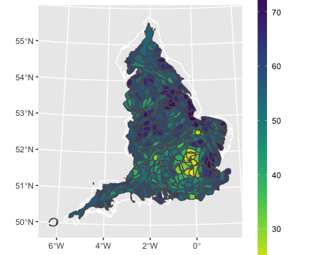
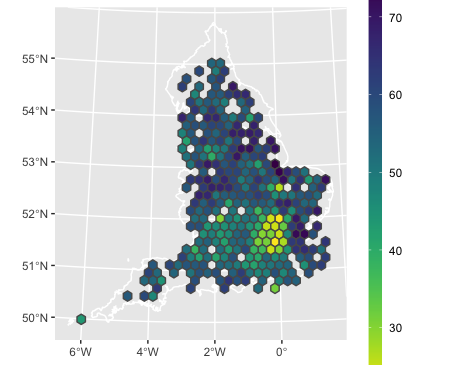
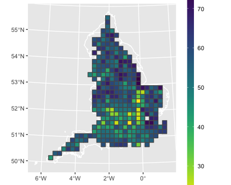
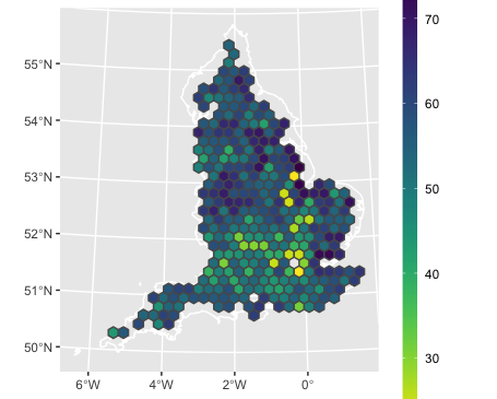
Results

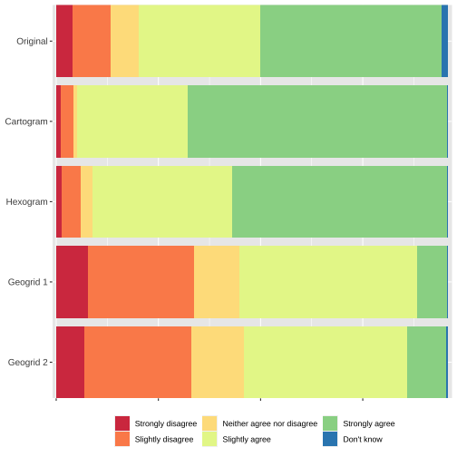
Results (contd.)

Conclusions

• New methods to visualise geographic information can convey a message more accurately than original thematic maps.

• But choose the method with consideration to the research question and the data!

Thanks!

• The paper: Langton, S. H., & Solymosi, R. (2019). Cartograms, hexograms and regular grids: Minimising misrepresentation in spatial data visualisations. Environment and Planning B: Urban Analytics and City Science.

• These slides: https://rekadata.net/talks/pydatamcr.html

• Questions? Contact myself (@r_solymosi) or Sam (@sh_langton)